standseg

Multi-resolution forest stand segmentation from satellite imagery, in Rust.

It implements the algorithm from Ye et al. (2025), which extends Harward and Woodcock's 1992 segmenter to take a second data layer. The original grows regions in one image and then forces the undersized ones to merge with whatever is nearest. The modification keeps that first stage as a micro-segmentation, and replaces the second with one that develops those micro-segments against a different image over the same grid: forest structure, age, or species over the same pixels.

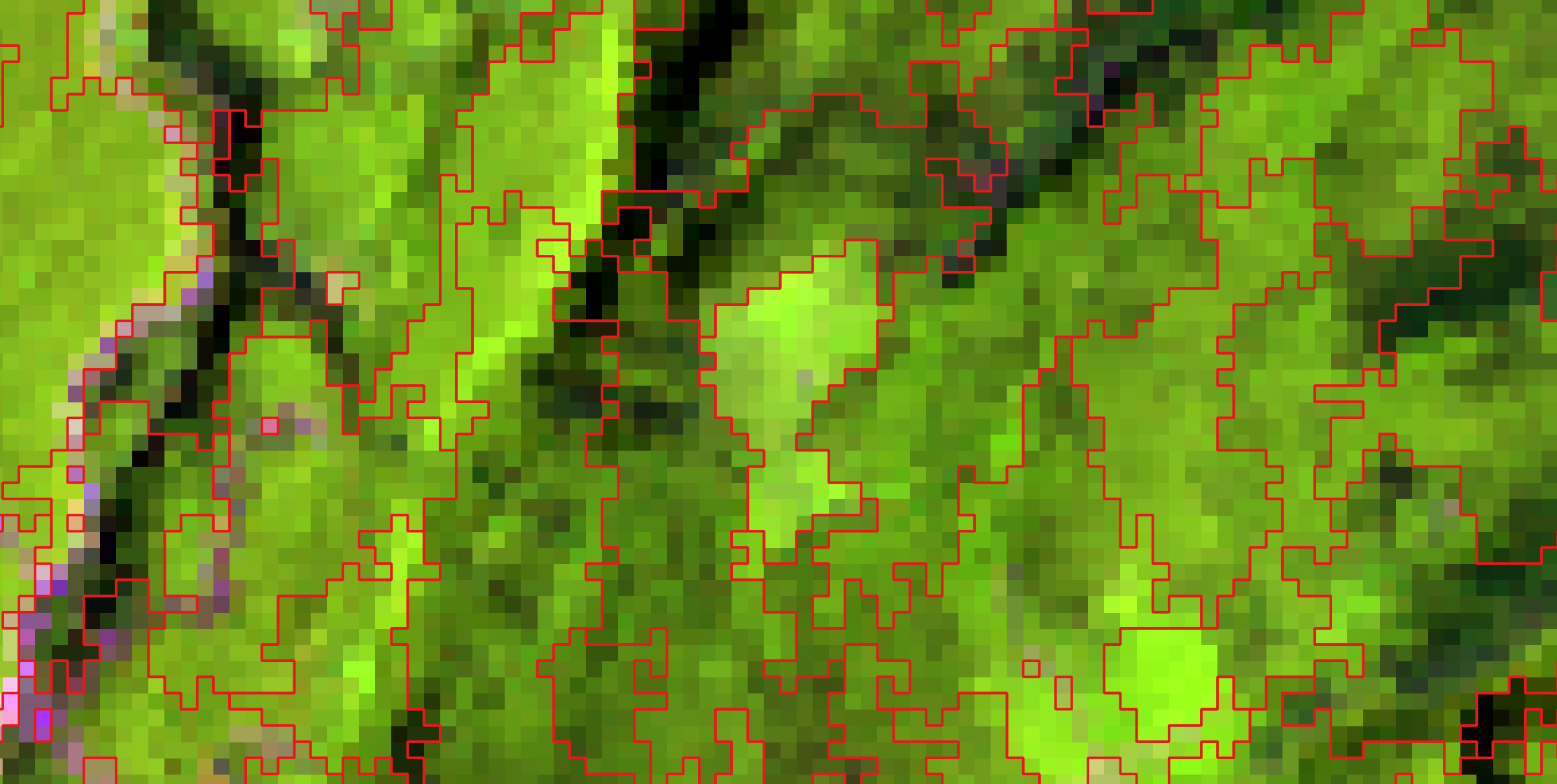
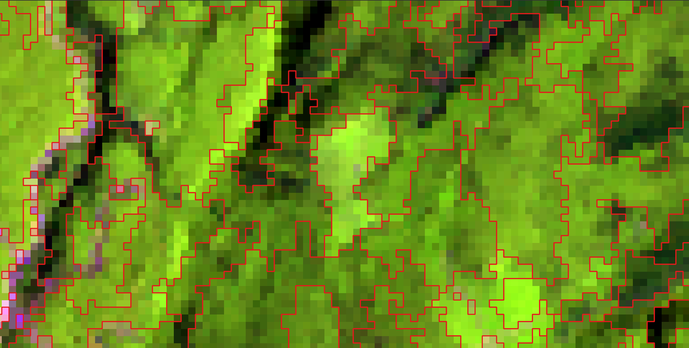
second layer: stand age	second layer: canopy height (elev_p95)

One Landsat scene, one phase 1, two second images. Phase 1 micro-segments the spectral proxies; phase 2 develops those micro-segments against the layer you give it, and the stands it draws are not the same ones. The second layers are NTEMS products — forest age and canopy height (elev_p95) — from the Canadian Forest Service and UBC; references under Licence.

The original algorithm is still in here and still exact. With one image the program does what the 1992 C did, byte for byte. The second layer is an option, not a fork, so both papers' methods run from the same binary.

It also handles images the C cannot — it segfaults above roughly 5000 × 5000 — and it is faster: 9.7 s where the original takes 24.5 s on a 5000 × 5000 tile, or 12.6 s if you rebuild the C with optimisation turned on, which its own Makefile does not.

This is for delineating forest stands from Landsat, and that is the only thing it has been validated on. The published results, the fixtures in this repository, and every byte comparison below are all Canadian forest tiles with Landsat spectral proxies and structure, age or species layers. Nothing stops you pointing it at other imagery, but I have not tested that and make no claim about it: the parameters, the size rules and the nodata convention were all chosen for stands, and I would not trust the output on another kind of scene without checking it against something you already believe.

I wrote the Rust with a coding agent, and the two old programs are what kept it honest. Every change was checked by segmenting the same image with the C, the Python and the Rust and comparing the output bytes, so "it looks right" was never the standard. Neither oracle is in this repository, but what they produced is: the fixtures under tests/golden/ and tests/stage2/ are their output, checksum-pinned, and cargo test re-runs the comparison on your machine. See How this was checked.

One scene, one command

A 250 x 250 Landsat subset ships inside the download, under sample/, so there is something to run on before you go and find data of your own. Unpack the archive, open a terminal in the unpacked folder, and:

# macOS and Linux
./standseg -t 20 -m .2 -n 50,100,200 --format gpkg -o stands --outdir out sample/temp_byte_bip

# Windows PowerShell -- note the .\ and the backslashes
.\standseg.exe -t 20 -m .2 -n 50,100,200 --format gpkg -o stands --outdir out sample\temp_byte_bip

Working from a clone instead of a release archive? The binary is target/release/standseg after cargo build --release, and the same scene is tests/golden/misc/temp_byte_bip.

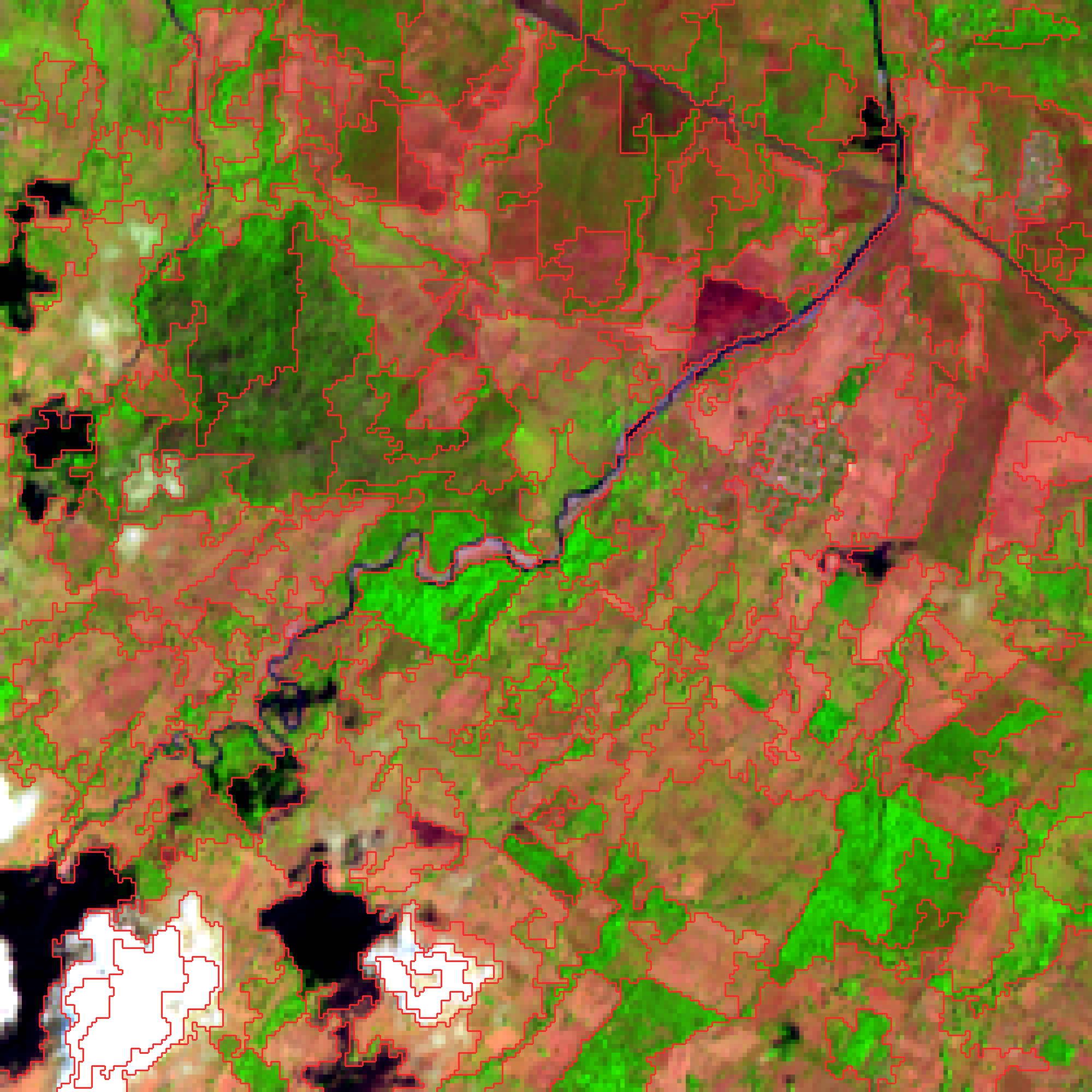
Landsat 8 OLI, WRS-2 path 22 / row 49, acquired 2014-03-24 (scene LC80220492014083LGN00): a 250 × 250 subset at 30 m in UTM zone 15N over Chiapas, Mexico, drawn here as a SWIR1/NIR/red composite. The red lines are the 163 stands standseg found, mean size 34.5 ha. Landsat data courtesy of the U.S. Geological Survey. python3 docs/make_figure.py out/stands.armap.69 redraws it.

Two maps come out, with the pass count in the name: out/stands.rmap.81.gpkg from phase 1 and out/stands.armap.69.gpkg from phase 2. --format gpkg makes them GeoPackages — one polygon per stand, which QGIS, ArcGIS, sf and geopandas open directly, and which you can also just query, because a GeoPackage is a SQLite database (if you have sqlite3 — QGIS is the easier route on Windows, where it is not installed by default):

$ sqlite3 -header out/stands.armap.69.gpkg \
    'SELECT region_id, n_pixels, area/1e4 AS ha FROM stands ORDER BY ha DESC LIMIT 3'
region_id|n_pixels|ha
29|1663|149.67
150|1536|138.24
124|1466|131.94

Leave --format off and you get ENVI rasters instead — the form every byte comparison here is against. Run the 1992 reference parameters and the bytes are identical to what the 1992 C produced. Its output is in sample/ too, so you can check that claim yourself rather than take it:

# macOS and Linux
./standseg -t 10 -m .1 -n 15,15,100,2500,2500 -o demo --outdir out sample/temp_byte_bip
cmp out/demo.rmap.51  sample/regmap.rmap.51
cmp out/demo.armap.58 sample/regmap.armap.58

# Windows PowerShell -- fc /b is the built-in byte comparison
.\standseg.exe -t 10 -m .1 -n 15,15,100,2500,2500 -o demo --outdir out sample\temp_byte_bip
fc /b out\demo.rmap.51  sample\regmap.rmap.51
fc /b out\demo.armap.58 sample\regmap.armap.58

cmp prints nothing and exits 0 when the files match; fc /b says FC: no differences encountered. Anything else is a bug in this program — see CONTRIBUTING.md. From a clone, cargo test --release runs that comparison and a good deal more.

Phase 1 merges mutually-nearest regions within the tolerance, one merge per region per pass, until a pass produces none. Phase 2 forces the regions still below the minimum size to merge, with no distance ceiling.

Those are not universal parameters — -t in particular is a raw DN distance and has to be scaled to your data. See Choosing -t before you trust a map.

Install

Download from the releases page, unpack, and run. One executable, no GDAL, no Python, no system libraries.

Linux	statically linked, so it also runs on older distributions and HPC login nodes
macOS	universal (Apple Silicon and Intel), signed and notarized, so it runs without a Gatekeeper warning
Windows	.zip, x86-64

There is no installer and nothing to add to PATH unless you want to. The program is one file that runs from wherever you unpacked it.

On Windows. Right-click the .zip → Extract All. Then open the extracted folder, shift-right-click in the empty space → Open PowerShell window here, and call the program as .\standseg.exe. Plain standseg will not work: it is not on PATH, and PowerShell does not look in the current directory. Two other things that catch people out — where a command below is split across lines with a trailing \, that is bash syntax, so join it into one line first — and if Windows blocks the first run with a "Windows protected your PC" banner, that is SmartScreen reacting to an unsigned executable from the internet (the macOS build is signed; the Windows one is not). Click More info → Run anyway, or right-click standseg.exe → Properties → tick Unblock.

On macOS. chmod +x standseg if your unpacker cleared the bit, then run ./standseg. It is signed and notarized, so there is no Gatekeeper prompt.

To call it from anywhere, put it somewhere already on PATH — sudo cp standseg /usr/local/bin/ on macOS or Linux; on Windows, move the folder somewhere permanent and add it under Edit environment variables for your account.

Anything else — or if you would rather build it:

cargo install --git https://github.com/Sugarc0de/standseg

That needs a Rust toolchain and a C compiler, because the GeoTIFF ZSTD support compiles a C library.

Every release binary is checked before it is published by segmenting the reference scene and comparing the result to the 1992 output byte for byte.

Segmenting with a second image

Add --stage2 and the same run micro-segments the first image, then develops the result against the second:

# one image -- Woodcock & Harward, unchanged
standseg -t 50 -m 0.2 -n 9,18,36 -o stands proxies

# two images -- the same run, plus segment development
standseg -t 50 -m 0.2 -n 9,18,36 \
    --stage2 elev_p95 --n2 80,8000 -o stands proxies

# or develop a stage-1 map you already have, against a different second image
standseg --rmap stands.rmap.41 --stage2 age --n2 60,8000 -o stands_age

The intermediate stands.rmap.41 is a real output, byte-identical to what the one-image run writes, so you can segment once and develop it several ways.

Three things about this phase are easy to trip over:

• A region merges with its nearest neighbour even when it is not that neighbour's nearest — the paper's relaxation, and the reason small segments get absorbed at all.
• The surviving id is the small region's, so ids in a --stage2 map are not comparable to a 1992 armap by id.
• A region more than half zero in the second image is dropped and zeroed. That is how non-treed area enters: the layers are rescaled to 1–255 with 0 reserved, so the mask comes from the second image rather than from -M.

The second image may be 32-bit float, which is how structural layers ship. The first may not — phase 1 works in integer DN, and that is enforced by the type system rather than a check that could be forgotten.

Segmenting a time series

standseg temporal segments a series of images over one grid. The first step is the two-image run above. At each later step only the pixels whose class changed are segmented again; those segments are pasted into the previous result and developed against that step's second image. Everything else carries forward.

# one row per step, in time order; `classes` is any categorical layer
# (land cover, burn severity, ...) whose change says what to redo
cat steps.csv
label,image,stage2,classes
2001,2001/proxies,2001/gsv,2001/landcover
2002,2002/proxies,2002/gsv,2002/landcover
2003,2003/proxies,2003/gsv,2003/landcover

standseg temporal --manifest steps.csv --normalize \
    -t 50 -m 0.2 -n 18,18,18,36,36 --n2 80,8000 -o site --outdir out

Rows are steps in time order. Columns are matched by name, and lines starting with # are ignored. Relative paths are read from the manifest's own folder, so a data folder can be moved together with its manifest. The label names each step's outputs and must be unique.

Real data rarely has one naming scheme across products. In that case, write the manifest with a short loop instead of by hand:

{
  echo label,image,stage2,classes
  for y in $(seq 1984 2022); do
    echo "$y,refl/SR_${y}_fitted.dat,struct/height_${y}.dat,landcover/LC_${y}_v2.dat"
  done
} > data/steps.csv

This writes out/site.<label>.armap.<passes> per step. To give the steps on the command line instead, repeat --image, --stage2 and --classes once per step. To supply change masks directly, give --change once per step after the first. --intermediates also writes each step's stage-1 map, change mask and combined map. The files of a series must share one grid; if they carry georeferencing, a file that is offset, has a different pixel size, or is in another coordinate system is refused. Every file is checked before the first step runs. --normalize rescales every input to 1–255 per band with nodata → 0, which is how the paper's inputs were prepared. standseg temporal --help has the rest.

Options

standseg --help lists all of them. The ones you will actually set:

Option	Meaning
-t <t1,t2,…>	Segmentation tolerance, in raw DN. Required. One map per value. See below.
-o <base>	Output basename. Required.
-n <a,b,c,d,e>	Nabsmin,Nnormin,Nviable,Nmax,Nabsmax — ascending, 0 means no limit.
-m <cm>	Merge coefficient. Caps merges per pass at cm × nregions.
--stage2 <image> / --n2 <min,max>	The second image and its size rules.
--rmap <file>	Start from a saved stage-1 map and skip phase 1.
--nodata <v>	Nodata value; may be negative (Landsat's -9999).
-M <file> / -8	Mask image; 8-way connectivity instead of 4-way.
-B <band> / -N <low,high>	Hold regions outside a normality interval to Nabsmin, so small non-forest patches are not absorbed.
--outdir / --format / --threads	Output directory; envi, tiff or gpkg; worker threads (output is identical either way).

The 1992 program stopped at 65535 in every -n position because its pixel counter was an unsigned short. That ceiling is gone; ask for -n …,65535,65535 if you want it back.

Choosing -t

This is the one parameter that will waste your afternoon, because getting it wrong does not produce an error. It produces a map.

-t is a distance in raw DN units. The published parameters (-t 50) are for layers rescaled to 0–255. Landsat Collection 2 ships 16-bit, where the same number means something roughly 250× smaller. On a 16-bit stack running 0–8990:

tolerance	first pass	regions in the final map
-t 10	merges almost nothing — 62 498 of 62 500 pixels stay separate	5 304
-t 350	merges normally — 55 056 of 62 500	3 983

At -t 10 the spectral phase is inert, the size rules force merges anyway, and you get a plausible-looking map that is 33 % off. Scale your tolerance by the ratio of the data ranges — 8-bit to 0–8990 is a factor of about 35, which is how -t 10 becomes -t 350. The program warns on stderr when it sees this, but the warning is a safety net, not a substitute for scaling the number.

Formats

Read ENVI, IPW, TIFF/GeoTIFF and PNG; write ENVI (default, byte-compatible with the original), TIFF, or GeoPackage polygons. Format is detected from content first, extension second — the 1992 reference input has no extension at all.

Samples may be uint8, uint16 or int16, and --stage2 also takes float32. The same values fed in at any integer width give bit-identical maps, so widening is a generalisation rather than a second algorithm. Wider integers and float64 are refused with a message naming the type.

Bands map to samples-per-pixel, so a 6-band satellite stack is 6 bands. A PNG alpha channel reads as an ordinary band and joins the spectral distance — use --nodata or -M for transparency instead.

Product packages are out of scope: a Landsat Collection 2 tar is not an input. This program takes a raster of values on a grid — the spectral bands, or a structural attribute layer over the same pixels. Unpacking a delivery, applying the scale factors and stacking the bands are jobs GDAL already does well. Build the stack first, then segment:

gdal_merge.py -separate -o proxies.tif LC08_..._B{2,3,4,5,6,7}.TIF

Nodata pixels get region 0, never join a region, never contribute to a centroid, and no region grows across them — without that, stands merge across lakes. In the validated runs the excluded pixels are non-treed area, which the layers carry as 0. The value comes from --nodata, else the file's own declaration (ENVI data ignore value, GeoTIFF GDAL_NODATA); an -M mask combines with either. A pixel is nodata when all bands match, since masked-to-land imagery carries 0 everywhere over water while a single-band 0 is ordinary dark ground; --nodata-any switches that.

Every map records the command that produced it, as ENVI history/software, TIFF ImageDescription/Software, or the GeoPackage layer description. There is no timestamp, on purpose: the same command twice gives byte-identical files.

Vector output

--format gpkg writes the region map as polygons rather than pixels, which is usually the point of segmenting in the first place. One feature per region:

column
region_id	the value the region carries in the raster map
n_pixels	pixels in the stand
area	n_pixels × the pixel area, in squared CRS units — divide by 10 000 for hectares in a metre-based CRS. Written only when the input is georeferenced, because a column of pixel counts labelled "area" is worse than no column

The polygons are the raster. Vertices land on pixel corners, nothing is smoothed or simplified, neighbouring stands share their vertices so there are no slivers and no gaps, and a stand's geometry area equals n_pixels × the pixel area exactly. A stand that -8 leaves in disjoint pieces is one multipolygon rather than several rows, and a stand with a hole in it gets a hole.

Georeferencing comes from the input — an ENVI map info or the GeoTIFF model tags — and becomes an EPSG code where one is derivable. An input with no georeferencing at all still writes, in pixel coordinates, and says so on stderr instead of implying a place.

One gap to know about: a CRS carrying no EPSG code survives from ENVI, where the coordinate system string is copied through as WKT, but not from GeoTIFF, where only the EPSG geokeys are read. Such a file gets correct map coordinates under srs_id −1, "undefined", and you will have to tell your GIS what the CRS is. Anything with an EPSG code — UTM, a national grid, plain WGS 84 — is unaffected.

Nodata gets no polygon: region 0 is left out of the layer rather than exported as one enormous multipolygon riddled with holes, so the features cover the segmented area and nothing else.

Phase 1 maps are big as vectors. A micro-segmentation is millions of tiny regions, and each one costs a geometry, a row and an index entry. On a 2500 × 2500 scene the phase-1 map is 2.2 M features and 473 MB against 134 k features and 130 MB for phase 2, and writing both as GeoPackage takes 9.9 s where the ENVI rasters take 5.4 s. Vectorise the phase-2 map; keep phase 1 as a raster.

Performance

M-series laptop, 10 cores, 6-band imagery:

scene	C, as its Makefile builds it	C, rebuilt -O2	this, serial	this, parallel
5000 × 5000	24.5 s	12.6 s	13.3 s	9.7 s
15000 × 15000	segfaults	segfaults	157.9 s	77.6 s

A 5000 × 5000 tile needs about 0.7 GB, 15000 × 15000 about 5 GB. The C fails above roughly 5000 × 5000 because ecalloc takes a signed 32-bit byte count and the centroid list overflows it.

Only the nearest-neighbour scan is parallel — the merge loop is inherently sequential — so expect about 2×, not one-per-core. That is the price of bit-exact output, and it is deliberate.

On a whole NTEMS tile (5000 × 5000 × 6 proxies, 5000 × 5000 × 1 elev_p95, paper parameters), one command with --stage2 takes 35.6 s and 1.20 GB, against 31.0 s and 1.17 GB for the one-image run. Phase 1 leaves 4 377 977 micro-segments; segment development takes them to 122 552 stands in 114 passes. The Python that defines that phase takes 14.5 s to the Rust's 0.28 s on a 1000 × 1000 crop, for byte-identical output.

How this was checked

A segmentation is hard to eyeball — two maps can look the same and be different everywhere it matters — so byte equality against a program that already worked was the rule for the whole rewrite. There were two such programs: the original C for the first phase, and my Python for the second.

Against the C. Both 1992 reference cases reproduce byte for byte in both phases, at the same pass numbers (51/58 and 17/1), with every per-pass statistic in the original's log matching. There is also a byte-identical run at 5000 × 5000, 400× the area of the test cases. The fixtures ship in tests/golden/, checksum-pinned and read-only, so cargo test --release re-runs the comparison on your machine.

Against the Python. Six generated cases in tests/stage2/ reproduce byte for byte, at the same pass counts and the same per-pass merge and rejection counts. Beyond those, four whole NTEMS tiles went through both implementations and were compared with cmp:

tile	second-stage layer	passes	result
397	6-band species, uint8	134	identical, 100 000 000 bytes
473	3-band structure, uint8	154	identical
474	1-band biomass, uint8	139	identical
219	3-band age, float32	130	identical

400 MB of region map, no differing bytes. The Rust runs took 21–26 s each; the Python took 1440–1780 s and 4.3–7.2 GB.

What does not reproduce. Both programs settle near-ties with a coin flip, and ties are not rare — on a single-band 8-bit layer close to half of all pixels have more than one nearest neighbour. The C's flip is random() & 01, never seeded, so it at least repeats. My Python called randint(0, 1) while iterating a set, which has no defined answer at all. So my 2023 second-phase maps cannot be regenerated from their own inputs, by me or by anyone, and I did not know that when I published. This version pins the rule — ascending region id, keep the incumbent on a near-tie — and under it the coin is never reached.

The honest summary for anyone publishing from this: the method reproduces, my specific 2023 maps do not, and from here on a run is repeatable. The two implementations disagree with those maps on the same pixels (about 1 % on single-band layers, 0.02 % on six-band), which is what a tie-driven difference looks like and is how I know it is the tie-break rather than a bug. The one part with no tie-break in it — the set of dropped nodata regions — matches the 2023 maps exactly, on all 52 experiments tested.

Over a time series. I re-ran the pipeline from my second paper here, with its helper code unchanged, on the three study sites I still have (39 years each). Every artifact of all 117 steps matched byte for byte: stage-1 map, change mask, combined map and final map. That is 461 MB with no differing bytes. A 39-year site takes 4–11 s here against 1–11 min in the Python. Four smaller cases ship in tests/temporal/. My archived 2024 runs of that pipeline reproduce in every step except the second phase, which was evidently run with code I never committed; PLAN.md §14.4 has the detail.

Repository layout

src/                  the segmenter
tests/golden/         1992 reference inputs and outputs, checksum-pinned
tests/stage2/         two-image segment-development fixtures, checksum-pinned
tests/temporal/       time-series fixtures, checksum-pinned
PLAN.md               design notes: algorithm, port hazards, memory, milestones
CONTRIBUTING.md       the rules the oracles impose; read before changing src/

Git does not preserve read-only permissions, so after cloning: tests/lock_golden.sh and tests/verify_golden.sh (and the _stage2 and _temporal equivalents).

Licence

MIT; see LICENSE. All of the code is my own — no third-party source is redistributed here.

The test data is not mine. The scene under tests/golden/misc/ is a subset of Landsat 8 LC80220492014083LGN00, a U.S. Government work in the public domain, courtesy of the U.S. Geological Survey. That subset, and the reference region maps under tests/golden/*/expected/proof/ that everything here is checked against, were assembled by Chris Holden and come from ceholden/segment, the extraction of the Harward–Woodcock code from IPW that this program was validated against. That repository states no licence terms.

The figures come from NTEMS, the National Terrestrial Ecosystem Monitoring System of the Canadian Forest Service and the University of British Columbia, distributed at opendata.nfis.org. No NTEMS data is redistributed here — the figures are renderings — but NTEMS asks that its products be cited, and the two second layers and the Landsat composites beneath them are its:

Matasci, G., T. Hermosilla, M. A. Wulder, J. C. White, N. C. Coops, G. W. Hobart, D. K. Bolton, P. Tompalski and C. W. Bater. 2018. Three decades of forest structural dynamics over Canada's forested ecosystems using Landsat time-series and lidar plots. Remote Sensing of Environment 216: 697–714.

Maltman, J. C., T. Hermosilla, M. A. Wulder, N. C. Coops and J. C. White. 2023. Estimating and mapping forest age across Canada's forested ecosystems. Remote Sensing of Environment 290: 113529.

Hermosilla, T., M. A. Wulder, J. C. White, N. C. Coops, G. W. Hobart and L. B. Campbell. 2016. Mass data processing of time series Landsat imagery: pixels to data products for forest monitoring. International Journal of Digital Earth 9(11): 1035–1054.

Citation

Which paper to cite depends on which half of the program you used.

• One image is Woodcock and Harward's algorithm, unchanged and byte-exact — Ye et al. contributed nothing to that path. Cite Woodcock & Harward.
• Two images (--stage2) is the segment development of Ye et al., built on Woodcock and Harward's phase 1. Cite both.

For the software itself, CITATION.cff carries the metadata GitHub and Zenodo read.

Ye, E., N. C. Coops, M. A. Wulder and T. Hermosilla. 2025. A multi-resolution forest stand segmentation algorithm integrating Landsat imagery and forest structural, age, and species attributes. ISPRS Journal of Photogrammetry and Remote Sensing. https://doi.org/10.1016/j.isprsjprs.2025.05.023

Woodcock, C. and V. J. Harward. 1992. Nested-hierarchical scene models and image segmentation. International Journal of Remote Sensing 13(16): 3167–3187.

Original algorithm and C implementation by Jud Harward and Curtis Woodcock, Boston University, building on the IPW library from UC Santa Barbara.